Gene Enrichment Analysis
Install packages
library(fgsea)
library(tidyverse)
Downloads genesets from the GSEA website
You can download the genesets that you are interested to check against your differentially expresssed genes from the website between. You can also creat a list of genes and their associated biological process function or components. The genesest is laoded as Mm.H object, class of the object is a list. You can make your own list.
load("Downloads/mouse_H_v5.RData")
class(Mm.H)
Now we are going to load our output from DESeq2 with contains, at least Entrez gene ID and log2FC. If your DESeq2 output has any other GeneID or Symbol you need to convert them to Entrez gene ID. I wrote about converting gene ID previously. But I also giving it here at the end of the analysis because our data already has Entrez gene ID.
load("Downloads/Annotated_Results_LvV.RData")
We now filter out any row that does not have Entrez gene ID.
gseaDat <- filter(shrinkLvV, !is.na(Entrez))
Make a rank vector of log2FC and set the name to Entrez Gene ID.
ranks <- gseaDat$logFC
names(ranks) <- gseaDat$Entrez
Sort the rank and look at the data as barplot.
ranks <- sort(ranks, decreasing = T)
barplot(ranks)
GSEA analysis
Now we can geneset enrichement analysis by using fgsea function of fgsea package. We are giving predefined geneset as list of genes and a named vector of log2FC. Name of log2FC vector is the Entrez gene ID.
fgseaRes <- fgsea(Mm.H, ranks, minSize=15, maxSize = 500, nperm=1000)
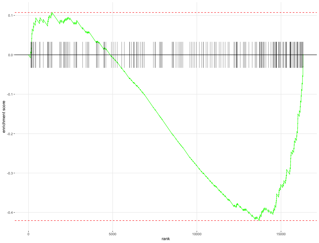
Now we can make an enrichment plot for our pathway of interest.
plotEnrichment(Mm.H[["HALLMARK_ESTROGEN_RESPONSE_EARLY"]], ranks)
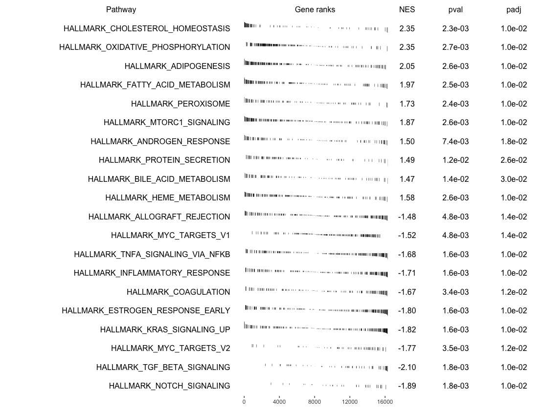
We can make GSEA table
topUp <- fgseaRes %>%
  filter(ES > 0) %>%
  top_n(10, wt=-padj)
topDown <- fgseaRes %>%
  filter(ES < 0) %>%
  top_n(10, wt=-padj)
topPathways <- bind_rows(topUp, topDown) %>%
  arrange(-ES)
plotGseaTable(Mm.H[topPathways$pathway],
              ranks,
              fgseaRes,
              gseaParam = 0.5)
Code for changing Ensemble gene ID to entrez gene ID
library(biomaRt)
mart <- useDataset("hsapiens_gene_ensembl", useMart("ensembl"))
genes <- getBM(
  filters="ensembl_gene_id",
  attributes=c("ensembl_gene_id", "entrezgene"),
  values=ensembl.genes,
  mart=mart)
ensembl.genes is a vector of your own genes of interest that you would like to convert.
KEGG Pathway Analysis
library(clusterProfiler)
library(pathview)
search_kegg_organism('mmu', by='kegg_code')

sigGenes <- shrinkLvV$Entrez[ shrinkLvV$FDR < 0.01 &
                                !is.na(shrinkLvV$FDR) &
                                abs(shrinkLvV$logFC) > 1 ]
sigGenes <- na.exclude(sigGenes)
kk <- enrichKEGG(gene = sigGenes, organism = 'mmu')
head(kk, n=10)

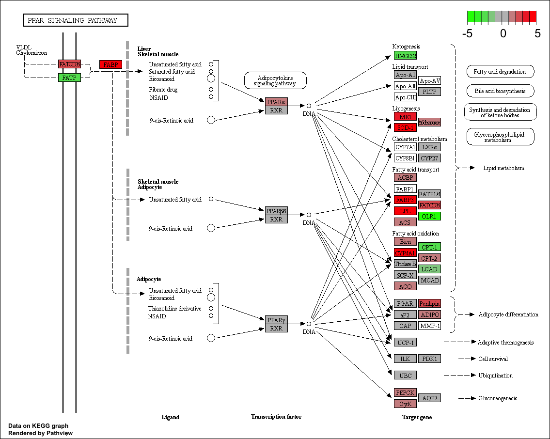
browseKEGG(kk, 'mmu03320')
setwd("~/Desktop/")
logFC <- annotLvV$logFC
names(logFC) <- annotLvV$Entrez
pathview(gene.data = logFC,
         pathway.id = "mmu03320",
         species = "mmu",
         limit = list(gene=5, cpd=1))
Gene Ontology Analysis
library(goseq)
supportedOrganisms() %>% filter(str_detect(Genome, "mm"))
isSigGene <- shrinkLvV$FDR < 0.01 & !is.na(shrinkLvV$FDR)
genes <- as.integer(isSigGene)
names(genes) <- shrinkLvV$GeneID
pwf <- nullp(genes, "mm10", "ensGene", bias.data = shrinkLvV$medianTxLength)
goResults <- goseq(pwf, "mm10","ensGene", test.cats=c("GO:BP"))
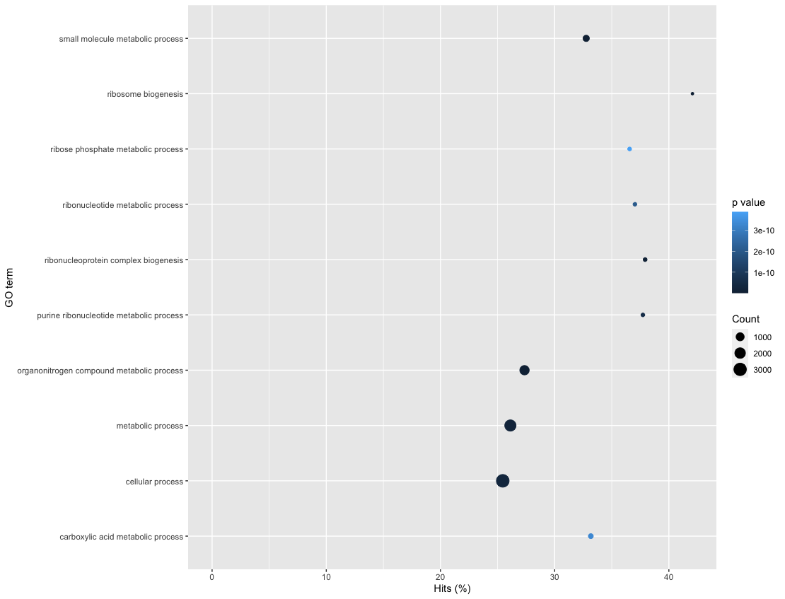
goResults %>%
  top_n(10, wt=-over_represented_pvalue) %>%
  mutate(hitsPerc=numDEInCat*100/numInCat) %>%
  ggplot(aes(x=hitsPerc,
             y=term,
             colour=over_represented_pvalue,
             size=numDEInCat)) +
  geom_point() +
  expand_limits(x=0) +
  labs(x="Hits (%)", y="GO term", colour="p value", size="Count")


