Creat necessary folders/directories

mkdir RNA_Seq_Analysis
cd RNA_Seq_Analysis
mkdir raw_data
mkdir fastqc_out
mkdir scripts
mkdir bam_files
mkdir count_file
mkdir meta_data

Download raw data from SRA

Go to following link and download accession list and metadata file. Accession list download link

Go to the link above and click on ‘Send to’(top right corner). Select “Run Selector” then click on ‘go’ Select above mentioned run then by clicking Metadata and Accession List we will get metadata and accession list file which we will use for our analysis. Accession list file name is SRR_Acc_List.txt and metadata file name is SraRunTable.txt. Move the acession list file to the raw data directory and SraRunTable.txt file to the metadata directory

cd raw_data
cat SRR_Acc_List.txt | xargs fastq-dump

Check quality of the raw data

We will use fastqc to check quality of raw data that we downloaded from sra database. The fastqc will generate html report of every file, I am not going to explain everything about those report but you can check this link to read about inpretation of fastqc report.

fastqc -o ~/RNA_Seq_Analysis/fastqc_out `ls *fastq`

Mapping raw data to the genome

Data we downloaded is RNA sequencing data from yeast strain between two different condition. In order to map this data to yeast genome I need to download yeast genome. I can download yeast genome using following command.

In order to consider sliced site I need to generate a file containing spliced site using extract_splice_sites.py script, which part of hisat2 software. Please download the hisat2

Generating index file from genome

cd scripts
wget ftp://ftp.ccb.jhu.edu/pub/infphilo/hisat2/downloads/hisat2-2.1.0-Linux_x86_64.zip
unzip hisat2-2.1.0-Linux_x86_64.zip

Download yeast fasta file for yeast genome.

cd annotation
wget ftp://ftp.ensembl.org/pub/release-99/fasta/saccharomyces_cerevisiae/dna/Saccharomyces_cerevisiae.R64-1-1.dna_sm.toplevel.fa.gz
gunzip Saccharomyces_cerevisiae.R64-1-1.dna_sm.toplevel.fa.gz

In order to reads to the genome, we need to make index of the genome using following command.

hisat2-build Saccharomyces_cerevisiae.R64-1-1.dna_sm.toplevel.fa Saccharomyces_cerevisiae.R64-1-1.dna_sm.toplevel

Generate splice sites

Download GTF file for yeast genome. You will need this file for generating known splice site and counting number of read align to the gene.

wget ftp://ftp.ensembl.org/pub/release-99/gtf/saccharomyces_cerevisiae/Saccharomyces_cerevisiae.R64-1-1.99.gtf.gz
gunizp Saccharomyces_cerevisiae.R64-1-1.99.gtf.gz

If you would like to perform a spliced alignment, you can provide a known spliced sites which hisat2 will use for alignment. You can make file with known splice site from gtf file using hisat2_extract_splice_sites.py scripts provided in hisat2 directory. Here I am using yeast gtf file, if you can use any gtf file you want.

python ./scripts/hisat2-2.1.0/hisat2_extract_splice_sites.py ./annotation/Saccharomyces_cerevisiae.R64-1-1.99.gtf > ./annotation/splicesites.txt

Alignment to the genome

Below is the code for aligning read to the yeast genome. My reads are single end therefore I have one fastq file as input. If you have paired end data you need to modify this code. You can run the code below from rawdata directory. The output for this code will be bam file in bam_file directory.

for fqfile in `ls *.fastq | sed 's/.fastq//g' | sort -u`
do
hisat2 -x ~/Documents/Tutorial/RNA_Seq_Analysis/annotation/Saccharomyces_cerevisiae.R64-1-1.dna_sm.toplevel --known-splicesite-infile ~/Documents/Tutorial/RNA_Seq_Analysis/annotation/splicesites.txt $fqfile.fastq | samtools view -Sb > ~/Documents/Tutorial/RNA_Seq_Analysis/bam_files/$fqfile.bam
done

Sorting BAM files

Before counting the code you need to sort the bam file by using samtools sort. Run code below from the bam_file directory. This will generate sorted.bam files.

for bam_file in `ls *bam | sed 's/.bam//g' | sort -u`;
do
samtools sort $bam_file.bam > $bam_file.sorted.bam
done

Indexing BAM file

If you would like visualize RNA-Seq data in IGV, you need to make an index file, below is the code for generating index file. After generating index file you can load sorted.bam file in IGV for visualization of RNA-Seq track.

for bam_file in `ls *sorted.bam`;
do
samtools index $bam_file 
done

Counting number of reads mapped to each feature

for bam_file in `ls *bam.sorted`;
do
featureCounts -s 2 -t exon -g gene_id -a ~/Documents/Tutorial/RNA_Seq_Analysis/annotation/Saccharomyces_cerevisiae.R64-1-1.99.gtf -o ~/Documents/Tutorial/RNA_Seq_Analysis/count_file/$bam_file ~/Documents/Tutorial/RNA_Seq_Analysis/bam_files/$bam_file
done

Differential gene expression analysis by R package DESeq2

Above code will generate file containing number of reads in each gene. Next of the RNA seq analysis is differential gene expression analysis by the R package DESeq2. Since next part we are going to use R package you need run code below in R studio.

Counts folder contain raw count data generated by featureCounts, there is one file for each sample. Sicne we have four sample we have four count files. In the first steps we are going merge all the file in one dataframe.

file_list <- list.files("~/Documents/Tutorial/RNA_Seq_Analysis/counts", pattern = 'bam.sorted$', full.name = TRUE)
counts_data <- read.table(file = file_list[1], header = TRUE)[,c(1,7)]
for (f in 2:length(file_list)){
  temp <- read.table(file = file_list[f], header = TRUE)[,c(1,7)]
  counts_file <- merge(counts_data, temp, by="Geneid")
}

We are changing column name of each sample, to make it look simpler and match with the metadata.

colnames(counts_file) <- c("Geneid", "SRR1761160", "SRR1761163", "SRR1761164", "SRR1761165")

Now we will create a dataframe to represent metadata, you can also input metadata from a file. Specifically the file we downloaded from runselector.

meta_data <- data.frame(sample=c("SRR1761160", "SRR1761163", "SRR1761164", "SRR1761165"),
                        condition=c("Nab2_depleted", "Nab2_depleted", "WT","WT"))

Next we will create an instance of deseqdatasetfrommatrix, which take following input: countData, which is the merged output from featureCounts, in our case is count_data object. colData, which is the information about the sample which is our case is meta_data object, design, which is how we would like to medel the sample that condition in our meta_data object.

dds <- DESeqDataSetFromMatrix(countData=counts_file, 
                              colData=meta_data, 
                              design=~condition, tidy = TRUE)

Before running the the deseq function if you would like to filter low counts genes you can run code below. This will filter out genes that have read counts less than 10.

keep <- rowSums(counts(dds)) >= 10
dds <- dds[keep,]

In order to determine differntially expressed gene between two condition describe in metadata, we can run deseq2 function.

dds <- DESeq(dds)
res <- results(dds)

Visualization of results

Visualization of log2 fold change data between wild type and Nab2 depleted strains by volcano plot.

with(res, plot(log2FoldChange, -log10(pvalue), pch=20, main="Volcano plot", xlim=c(-3,3)))
with(subset(res, padj<.05 ), points(log2FoldChange, -log10(pvalue), pch=20, col="blue"))
with(subset(res, padj<.05 & abs(log2FoldChange)>2), points(log2FoldChange, -log10(pvalue), pch=20, col="red"))

Here is the volcano plot:

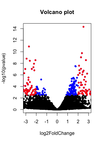
Volcano plot

If we have multiple samples we can visualize log2FoldChange by using clustering and heatmap. Letter tutorial I will write about making heatmap in R.